The Toxic Link: Lead Exposure & Violent Crime in Chicago

Overview
This group project investigates the relationship between childhood lead exposure and violent crime rates across Chicago neighborhoods, with a 15-year temporal lag applied to reflect the neurological development timeline between early-life lead poisoning and its behavioral outcomes in adulthood. Using publicly available data from the Chicago Data Portal and Kaggle, the project combines data engineering, statistical analysis, and data visualization to surface a striking correlation (Pearson's r = 0.581, p < 0.001) between historic lead exposure levels and violent crime counts at the community area level.
The work was completed for a data visualization course in which each team member took ownership of a distinct visualization component. This page documents my individual contributions.
Role & Contributions
My responsibilities centered on the statistical analysis and correlation visualization component of the project. Specifically, I was responsible for:
- Assessing the shape and distribution of the lagged data to inform visualization decisions
- Applying an appropriate data transformation to address skew and zero values
- Computing descriptive summary statistics to audit data quality and justify design choices
- Running a Pearson correlation test and extracting r and p-values for annotation
- Building the final regression scatter plot using ggplot2, with visual encoding by year and statistical annotation
The files I produced for this component were the R script (chicagocrime.R) and the final correlation scatter plot (leadExposureVsViolentCrime.png).
Sources
- City of Chicago. (2014). Public Health Statistics - Screening for elevated blood lead levels in children aged 0-6 years by year, Chicago, 1999–2013. Chicago Data Portal.
- City of Chicago. (2024). Chicago Crime [Data set]. Kaggle.
Tools & Technology
- R – Primary analysis environment
- ggplot2 – Scatter plot, regression line, and theme
- dplyr – Summary statistics and data wrangling
- colorspace – Sequential color palette for year encoding
- Base R (cor.test) – Pearson correlation and p-value extraction
The broader project also used Python (pandas) for the ETL pipeline, React/HTML for the slide presentation, and Power BI for an interactive dashboard — these were owned by other team members.
Methodology
4a. Exploratory Visualization & Justifying the Log Scale
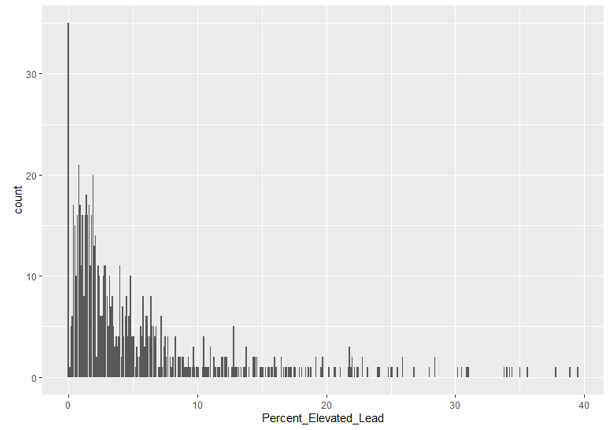
Before building the final chart, I produced a simple bar distribution of the raw Percent_Elevated_Lead variable using geom_bar(). The plot immediately revealed a heavily right-skewed distribution — a large number of community areas clustered near zero with a long tail of high-exposure outliers. This initial diagnostic visualization, combined with the summary statistics (see below), made clear that plotting the raw values would compress most of the data into an unreadable range and allow extreme outliers to dominate the visual.
4b. Data Transformation
To address the skew, I applied a log1p transformation (log1p(x) = log(1 + x)) to both the lead exposure and crime count variables. The choice of log1p over the more common log10 was deliberate: the raw data contained true zero values (community areas with no recorded elevated lead cases in a given year), and log(0) is undefined. log1p shifts the input by 1 before taking the log, preserving zeros as 0 in the transformed space and avoiding data loss or imputation.
Raw data → log1p transformation: log(1 + x) → Transformed variables ready for analysis
4c. Summary Statistics & Data Quality Audit
With the transformed variables in hand, I computed a comprehensive summary statistics table using dplyr::summarise(), capturing N, mean, median, standard deviation, variance, and maximum for both the lead and crime variables. This served as a data integrity check — verifying row counts, identifying the magnitude of spread, and confirming the extreme range between median and maximum values that had initially warranted the log scale. The large gap between median and max in the raw data (e.g., a median lead percentage near 2–3% but a maximum near 22–24%) validated that the log transformation was the appropriate corrective step rather than simply clipping outliers.

4d. Correlation Testing
I used R's cor.test() on the log-transformed variables to compute the Pearson correlation coefficient and associated p-value. The raw p-value returned by R was 1.150112e-70 — scientifically precise but meaningless to a general audience. Rather than displaying this number, I used the industry-standard threshold label p < 0.001, which communicates statistical significance clearly without implying false precision. The r-value was rounded to three decimal places (r = 0.581) and both values were embedded directly into the plot as annotations.
4e. Final Visualization
The scatter plot was built in ggplot2 with the following design decisions:
- Regression line: geom_smooth(method = "lm") adds a linear model fit with a shaded 95% confidence interval, providing a visual anchor for the correlation trend.
- Color encoding: Points are filled by Crime Year using colorspace's scale_fill_continuous_sequential(palette = "Blues"), a perceptually uniform sequential palette that clearly differentiates years without introducing misleading categorical boundaries.
- Point aesthetics: shape = 21 (circle with separate fill and stroke), a grey border (color = 'grey20', stroke = 0.5), and alpha = 0.5 transparency allow overlapping points to remain individually visible while the density of the cloud communicates data concentration.
- Annotation placement: The statistical annotation (r and p-value) was positioned at x = max, y = min with hjust = 1 and vjust = 0, anchoring it to the lower-right corner of the plot where the data is sparse — avoiding overlap with the regression line or point cloud.
Challenges & Learnings
Right-skewed data and knowing when to transform
The most consequential analytical decision in this project was recognizing that the raw data needed transformation before visualization. My first step — plotting a simple bar chart of the raw distribution — gave me an immediate, visual justification for the log scale rather than relying on intuition alone. Pairing that diagnostic plot with summary statistics (particularly the divergence between median and maximum values) gave me both the evidence and the explanation to justify the transformation clearly to an audience.
log1p vs. log10
The presence of zeros in the dataset was a subtle but important constraint. log10(0) is undefined, which would silently drop data points or produce errors. Using log1p was the correct solution, and understanding why — the mathematical shift that makes zero a valid input — deepened my practical understanding of when each transformation is appropriate.
Communicating p-values to a general audience
R returned a p-value of 1.150112e-70 — technically accurate but effectively unreadable in a slide presentation. Displaying p < 0.001 is the established convention in data journalism and academic publishing for values below the threshold of practical interpretation. This was a small but meaningful lesson in the difference between statistical output and statistical communication.
Annotation placement with hjust/vjust
Getting the r and p-value label to sit in a clean, unobstructed part of the plot required understanding how ggplot2 handles text justification relative to anchor coordinates. Setting hjust = 1 (right-aligned) and vjust = 0 (bottom-aligned) at the maximum x and minimum y coordinates placed the annotation neatly in the lower-right corner.
Aesthetic polish
The default ggplot2 color scales were functional but visually flat. Switching to colorspace's sequential "Blues" palette produced a smoother, more professional gradient. Adding a visible point outline (shape = 21 + grey stroke) and partial transparency (alpha = 0.5) transformed a cluttered point cloud into a readable visualization where overlap is visible rather than obscured.
Outcome
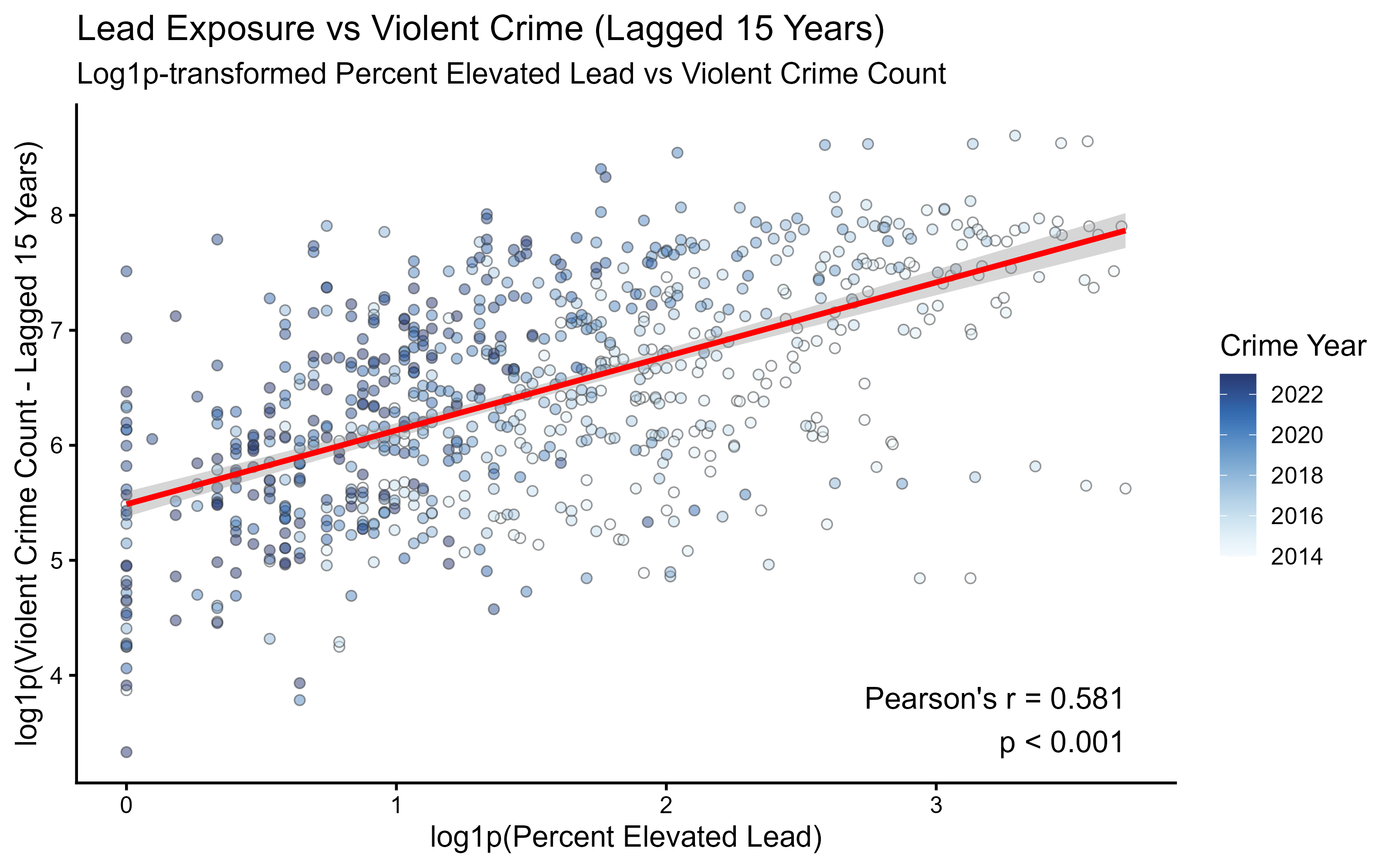
The final scatter plot demonstrates a statistically significant positive correlation between log-transformed childhood lead exposure and violent crime counts across Chicago community areas, lagged 15 years (Pearson's r = 0.581, p < 0.001). The visualization was integrated into the team's final slide presentation alongside trend charts, a neighborhood comparison, and an interactive Power BI dashboard.
Beyond the course deliverable, this project reinforced a workflow I now apply consistently: always interrogate the raw distribution before visualizing it, let summary statistics drive design decisions, and translate statistical outputs into language that serves the audience rather than the software.
GitHub Repository: github.com/mlingley/LeadCrimeProject